
Excel: Visa oskyddade celler
I den här artikeln kommer du att lära dig att färga visa oskyddade celler i Excel.
Formeln för framgång - så kan du visa oskyddade celler i Excel
- Öppna Excel-dokumentet där du vill visa de oskyddade cellerna. Välj sedan området där du vill visa de oskyddade cellerna.
- Klicka på fliken "Start" och välj posten "Villkorlig formatering". Klicka sedan på "Ny regel" i snabbmenyn.
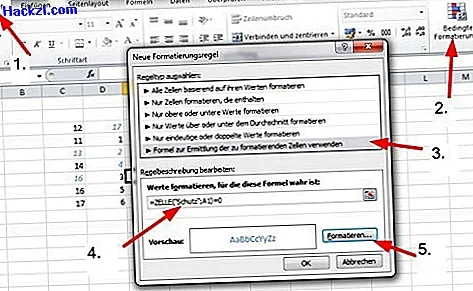
- Ett fönster öppnas med namnet "Ny formateringsregel". Välj regeltyp "Använd formel för att bestämma celler som ska formateras".
- Under "Formatera värden för vilken denna formel är sant:" ange formeln = CELL ("Skydd"; A1) = 0. Klicka sedan på "Format ..." och välj en färg där oskyddade celler ska visas.
- Klicka på "OK" för att tillämpa inställningarna. Kort därefter visas de oskyddade cellerna.
Det praktiska tipset visar var du kan hitta andra användbara Excel-övningar.